Graph Sketching and Interpretation for the ESAT

Linear Functions

The most fundamental graph is the linear function, which always results in a straight line. It is commonly expressed in the form $y = mx + c$. In this equation, $m$ represents the gradient (the steepness of the line) and $c$ represents the $y$ intercept, which is the point where the line crosses the vertical axis.

Quadratic Functions

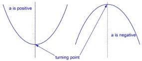
A quadratic function takes the form $y = ax^2 + bx + c$. Its graph is a curve known as a parabola, which is often described as u-shaped. The constant $c$ identifies the point where the curve intersects the $y$ axis.

The orientation of the curve depends on the coefficient $a$:

1. If $a > 0$, the curve is $\cup$ shaped (opening upwards).
2. If $a < 0$, the curve is $\cap$ shaped (opening downwards).

Every quadratic graph has a vertical line of symmetry and a single turning point. You can find the coordinates of this turning point by completing the square. The points where the curve crosses the $x$ axis, known as the roots, are found by solving the equation $ax^2 + bx + c = 0$.

Simple Cubic Functions

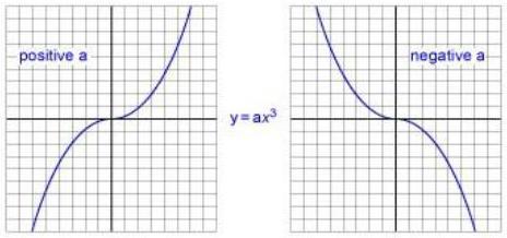
Basic cubic functions of the form $y = ax^3$ have a distinct shape that possesses rotational symmetry of order 2 about the origin $(0,0)$. This means if you rotate the graph 180 degrees around the origin, it remains unchanged.

Reciprocal Function

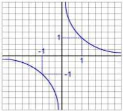
The reciprocal function is defined as $y = \frac{1}{x}$, where $x \neq 0$. Because division by zero is undefined, the graph never touches the $y$ axis. Similarly, since the fraction can never equal zero, it never touches the $x$ axis.

Key characteristics include:

1. When $x$ is positive, $y$ is positive. When $x$ is negative, $y$ is negative. Therefore, the curve exists only in the first and third quadrants.
2. The graph passes through specific points such as $(1, 1)$ and $(-1, -1)$.
3. As $x$ increases in value, $y = \frac{1}{x}$ decreases, approaching zero.
4. As $x$ gets closer to zero, $y = \frac{1}{x}$ becomes very large.

The Exponential Function

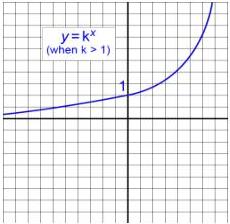
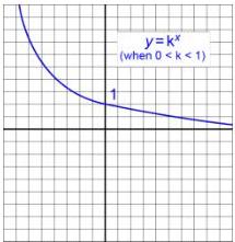
The exponential function is written as $y = k^x$, where $k$ is a positive constant. All such functions pass through the point $(0, 1)$ because any positive number raised to the power of zero equals one.

When $k > 1$: As $x$ increases, $y$ increases rapidly. For negative values of $x$, the value of $y$ lies between 0 and 1, getting closer to zero as $x$ becomes more negative.

When $0 < k < 1$: As $x$ increases, $y$ decreases rapidly. For negative values of $x$, the value of $y$ increases as $x$ becomes more negative.

Trigonometric Functions

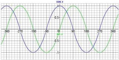
Trigonometric functions for any angle size (measured in degrees) exhibit periodic behaviour. The functions $\sin \theta$ and $\cos \theta$ both oscillate between a maximum of $+1$ and a minimum of $-1$.

Key values to remember:

1. $\sin 0^\circ = 0$ and $\sin 90^\circ = 1$.
2. $\cos 0^\circ = 1$ and $\cos 90^\circ = 0$.

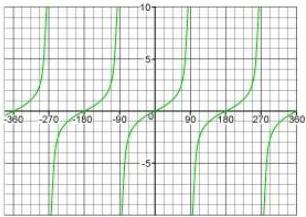
The function $\tan \theta$ behaves differently, varying between $-\infty$ and $+\infty$. It has a value of 0 at $0^\circ$ and has vertical asymptotes where the function is undefined, such as at $90^\circ$.

Worked Example: Comparing Power Functions

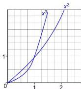
Consider the task of sketching $y = x^2$ and $y = x^3$ for the interval $0 \leq x \leq 2$ on the same axes.

At $x = 0$, both functions equal 0. At $x = 1$, both functions equal 1. To interpret the graph between these points and beyond:

1. For $x > 1$, the cubic grows faster: $x^3 > x^2$. For example, if $x = 2$, $2^3 = 8$ while $2^2 = 4$.
2. For $0 < x < 1$, the square is actually larger: $x^3 < x^2$. For example, if $x = 0.5$, $0.5^3 = 0.125$ while $0.5^2 = 0.25$.

Worked Example: Intersections

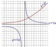
How many times do the graphs of $y = \frac{1}{x}$ and $y = 2^x$ touch or cross? By sketching both curves on the same set of axes, we can see the reciprocal curve in the first quadrant and the exponential growth curve. The exponential curve starts at $(0, 1)$ and increases, while the reciprocal curve decreases from very high values as $x$ increases from zero. They cross exactly once.

Worked Example: Trigonometric Inequalities

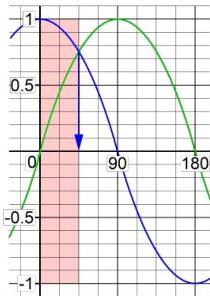
Find the range of values for which $\sin \theta < \cos \theta$ in the interval $0 \leq \theta \leq 180^\circ$.

First, sketch both $\sin \theta$ and $\cos \theta$. At $\theta = 0^\circ$, $\sin 0^\circ = 0$ and $\cos 0^\circ = 1$. The curves intersect when $\sin \theta = \cos \theta$, which occurs at $\theta = 45^\circ$ in this range. By looking at the sketch, the sine curve is below the cosine curve from the start until they meet. Therefore, the range is $0 \leq \theta \leq 45^\circ$.