Radioactive Half life for the ESAT

Updated July 2026

Master the concept of half-life for the ESAT Physics section. You will learn to define half-life, interpret decay graphs for parent and daughter nuclei, and perform precise calculations involving activity, time, and background radiation. A critical fact is that half-life remains constant regardless of sample size or external conditions.

Core concept

The half-life of a radioactive isotope is the average time taken for half of the nuclei in a sample to decay, or the average time taken for the count rate to decrease to half its initial value.

Understanding the Meaning of Half life

Radioactive decay is a random and spontaneous process, meaning we cannot predict exactly when a specific nucleus will decay. However, for a large number of nuclei, the rate of decay is highly predictable. The half-life is the primary measure used to describe this rate. Because the count rate (activity) of a source is directly proportional to the number of unstable nuclei remaining, the time taken for the count rate to halve is identical to the time taken for half the nuclei to decay.

Different isotopes possess vastly different half-lives, ranging from fractions of a second to billions of years. Crucially, the half-life of a particular nuclide is a constant: it is not affected by the size of the sample, the age of the sample, or external factors such as temperature or pressure.

Example: Factors affecting half-life Which of the following affects the half-life of a sample of a radioactive nuclide?

The number of unstable atoms in the sample.
The length of time for which the sample has been decaying.
Which radioactive nuclide is present in the sample.

Solution: Half-life is a fundamental property of the specific nuclide (isotope). It does not change as the sample gets smaller or as time passes. Therefore, only option 3 is correct.

Interpreting Graphical Representations

The half-life can be determined from a graph of count rate against time. You choose any starting count rate, find its corresponding time, and then find the time at which the count rate has fallen to half of that value. The difference between these two times is the half-life.

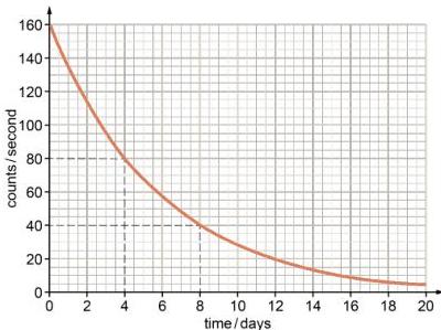
In the graph above, the count rate drops from $160$ cps (counts per second) to $80$ cps in $4$ days. If we check again from $80$ cps to $40$ cps, the time interval is from day $4$ to day $8$ , which is another $4$ days. This confirms the half-life is $4$ days.

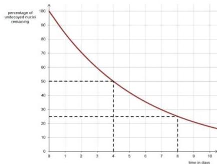
We can also plot the percentage of undecayed nuclei remaining. This graph follows the same exponential decay curve. At $t = 0$ , $100\%$ of the nuclei are undecayed. After one half-life, $50\%$ remain. After two half-lives, $25\%$ remain.

Consideration of Decay Products

When a parent nuclide (X) decays, it often turns into a stable daughter nuclide (Y). If we assume all atoms stay within the sample, the total percentage of nuclei (X + Y) must always equal $100\%$ . As the percentage of parent nuclei decreases, the percentage of daughter nuclei increases symmetrically.

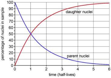
At the point where the two lines cross, the sample contains $50\%$ parent nuclei and $50\%$ daughter nuclei, which corresponds exactly to one half-life.

Worked Examples: Finding Half life from Graphs

Example 1: Percentage remaining The graph below shows the percentage of undecayed nuclei remaining against time. Find the half-life.

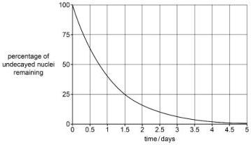
Solution: To improve accuracy, we can look for the time taken to halve twice. At $t = 0$ s, we have $100\%$ . The percentage falls to $25\%$ at $t = 1.5$ s. Since $25\%$ represents two half-lives, one half-life is $1.5$ s divided by $2$ , which is $0.75$ s.

Example 2: Uncorrected count rate and background The graph below shows measurements not corrected for background radiation. Find the half-life.

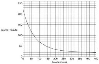
Solution: The graph levels off at $20$ cpm (counts per minute), which is the background count rate. At $t = 0$ min, the total rate is $220$ cpm, so the source rate is $220 - 20 = 200$ cpm. We need the source rate to halve to $100$ cpm. The total measured rate at that time will be $100 + 20 = 120$ cpm. Looking at the graph, the total rate is $120$ cpm at $t = 50$ min. Thus, the half-life is $50$ minutes.

Half life Calculations

If you know the half-life and initial count rate, you can predict future or past activity using the following logic: count rate halves every half-life going forward, and doubles every half-life going backward.

Worked Example: Count rate predictions A radioactive source has a half-life of $10$ seconds. Its current measured count rate is $64000$ cps.

a. What was the count rate $20$ s ago? Solution: $20$ s is two half-lives. Moving backward, we double the rate twice: $64000$ to $128000$ to $256000$ cps.

b. What will the count rate be after $30$ s? Solution: $30$ s is three half-lives. Moving forward, we halve the rate three times: $64000$ to $32000$ to $16000$ to $8000$ cps. Alternatively, calculate $(\frac{1}{2})^3 \times 64000 = 8000$ cps.

c. After how much time will the count rate be $500$ cps? Solution: Determine how many halvings are needed to reach $500$ from $64000$ : $64000$ to $32000$ to $16000$ to $8000$ to $4000$ to $2000$ to $1000$ to $500$ . This is $7$ halvings. Since each half-life is $10$ s, the total time is $7 \times 10 = 70$ s.

Key takeaways

Half-life is the constant average time taken for half of a radioactive sample's nuclei to decay.
The count rate of a source is proportional to the number of undecayed nuclei remaining.
To find the true source activity, the background count rate must be subtracted from the total measured count rate.
On a decay graph, the parent and daughter percentages always sum to 100% at any given time.
Calculations involve halving the activity for every half-life passed or doubling it for every half-life going back in time.

Tips

In ESAT questions, look for easy-to-read points on a graph, such as the y-intercept or the point where the value reaches 25% or 12.5%. This often allows you to calculate the half-life more accurately than just looking at the 50% point.

Cautions

The most common error is forgetting to subtract the background radiation from total count rate readings before performing any halving calculations. Always check the baseline of a graph to see if it reaches zero or levels off at a background value.

Insight

Half-life is mathematically linked to the decay constant. Although individual decays are random, the probability of decay per unit time is constant for a given isotope, which results in the characteristic exponential decay curve seen in all radioactive substances.

Frequently asked questions

Can half-life be used to predict when a single specific nucleus will decay?

No. Radioactive decay is a random process. Half-life is a statistical measure that applies to large groups of nuclei, not individual atoms.

What happens to the total mass of the sample as it decays?

While the number of parent nuclei decreases, they are replaced by daughter nuclei. The mass number changes only in alpha decay (by -4) and stays the same in beta decay, so the overall mass of the sample changes very little, though its composition changes significantly.

Why must we subtract background radiation before calculating half-life?

Background radiation is constant and not related to the source. If it is not subtracted, the measured count rate will never actually halve, leading to an incorrect and increasingly exaggerated calculation of the half-life.

Is there a formula for the number of nuclei remaining after $n$ half-lives?

Yes. The number of remaining nuclei $N$ can be calculated from the initial number $N_0$ using $N = N_0 \times (\frac{1}{2})^n$ , where $n$ is the number of half-lives elapsed.

Ready to test your knowledge?

You've reached the end of this section. Start a practice session to solidify your understanding and master this topic.

Ionising Radiation Penetration Ionisation And Background